In another post we have defined what a strongly perturbed physical system is. This implied that we know how to do strong perturbation theory, that is, one takes her preferred differential equation and get a solution series for the case of a large parameter. We show here that is indeed the case. So, let us consider as an example the following differential equation:
 .
.
We know the exact solution of this equation being

to be compared to our approximated ones. The weak perturbation case,  , asking for a solution in the form

gives the set of equations


and finally

and from the numerical comparison for  we get the curves

that is really satisfactory. We now look for a solution series in the form

but a direct substitution into the original equation gives nonsense. There is one more step to do and this is a rescaling in time, that is we use instead of  the scaled variable
  . After this substitution is accomplished we can put the strong perturbation series into the equation and obtain the meaningful set of differential equations


where now “dot” means derivation with respect to  . We have finally the solution series, undoing the rescaling in time,

Numerical comparison with  gives
gives

that is almost perfect in the coincidence between the exact and the approximate case. The method indeed works!
We note the following:
- From the set of equations of the strong perturbation case we note that we have just interchanged the perturbation with respect to the weak perturbation case to obtain the series with inverted expansion parameter. This serves just as a bookeeper but it is not needed. This is duality in perturbation theory (look here and here).
- The strong perturbation series is a series in small times. Indeed the time scale is set by
 that decides how far can we go into the time scale for the comparison.
It is just curious that no mathematician in the history was able to get such a method out understanding that it was just a rescaling of the independent variable away. I was lucky as this did not happen!
So, as said at the start, you can take your preferred differential equation and sort out a solution series in a regime you have never seen before.
Have fun!


 Posted by mfrasca

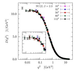
 a constant and
  the mass gap entering into the fit. We obtain the following figure
 and
and  . This result is really shocking. The reason is that a resonance with this mass has been indeed observed. This is


 . So, one has
  . The solution of this set of differential equations gives all one needs to obtain observables, that is numbers, to be compared with experiments. When the physical system undergoes the effect of a perturbation
  the problem to be solved is
 .
. is considered and the solution series we look for has the form
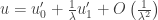 .
.

