What about ghosts?

As most of my readers know, in order to quantize Yang-Mills field one has to introduce a ghost. This result is due to Fadeev and Popov and since then, technology to work out high-energy behavior of QCD has been widely known. When you have a field you will also have a propagator as also unphysical degrees of freedom, as the ghost is, do propagate. But, in the end of your computations, all these contributions magically disappear giving a meaningful result. When you do your high energy computations you will have as a bare ghost propagator the one of a free particle but this field behaves quite strangely violating spin-statistic theorem. The main question we are concerned here is: How does ghost propagator behave in the infrared (low-energy) limit? Some researchers proposed that this propagator should go to infinity faster than that of a free particle (enhancement): This has been dubbed scaling solution . You  can read a nice paper about by Alkofer and von Smekal describing this kind of solution (see here). Lattice simulations went otherwise. In order to have an idea you can read a paper by Cucchieri and Mendes (see here) that shows, at a leading order of small momenta, that the ghost propagator, in the low-energy limit, is that of a free particle! This kind of solution has been dubbed decoupling solution.

Alike Alkofer and von Smekal, other authors thought to use Dyson-Schwinger equations to get the infrared behavior of such quantities like the ghost propagator. A French group, Boucaud,  Gomez ,  Leroy,  Le Yaouanca,  Micheli, Pene, Rodriguez-Quintero, has produced a lot of important papers showing how decoupling solution indeed comes out. I should say that I am an enthusiastic fan of this group as their results coincide perfectly with my findings. They work mostly numerically on lattice and solving Dyson-Schwinger equations also using interesting theoretical approaches. Quite recently, they put out a beautiful paper (see here) where they solve Dyson-Schwinger equation for the ghost propagator but using a smart trick to make it independent from the one of the gluon propagator. They just take the simplest hypothesis for a gluon propagator

(this is exactly the first term of my propagator!), than they show that the solution for the ghost propagator goes like a free propagator plus a logarithmic correction at higher momenta that they are able to compute.  This solution coincides quite perfectly with lattice computations. Gluon mass is seen to be around 500 MeV as it must be (that is also my case). So, a massive propagator (or a massive gluon) implies necessarily a decoupling solution as is seen on lattice computations. This conclusion is quite striking but is not enough. To have a clear idea of this finding one needs to understand what happens, with such an ansatz, to the scaling solution. This has been obtained in a paper appeared today by Rodriguez-Quintero (see here). The conclusion is again striking: A scaling solution emerges only for a critical coupling when enhancement is asked for in the ghost propagator. This, at best, means that this solution is atypical and this gives also a hint why is not seen on lattice computations for 3d and 4d. I would like to remember that the scaling solution appears in lattice computations in 2d when Yang-Mills theory is trivial and has not dynamics. It would be interesting to add similar terms to their ansatz for the gluon propagator: They should be able to recover my gluon propagator with the right spectrum to be compared with quenched lattice computations for QCD.

These results are really shocking but I should say that most has yet to be done on the way to get a complete understanding of Yang-Mills theory. Papers analyzing both scaling and decoupling solutions are fundamental to learn the relevance of such solutions and how they can come out. Presently, decoupling solution is strongly supported by lattice computations and several theoretical works, not last my papers, and I hope that future analysis could hopefully decide for the right scenario.

Triviality

One of the questions that is not that easy to answer is: When is a quantum field theory exactly solved? Of course, we have the example of a free theory. When one is able to put the generating functional into a Gaussian form, the spectrum of the theory is that of a harmonic oscillator and when the coupling is zero, one is left with a possibly solved theory. But this case is trivial and does not say anything about the case of an exactly solved but interacting quantum field theory. An immediate answer to this question is: When one is able to get all the n-point functions. This implies that, if you are able to solve all the hierarchy of Dyson-Schwinger equations, you are done. Solving this set of equations is practically impossible in almost all the interesting case. But there is an exception and a notable one. So, consider the case of a massless quartic scalar field theory. Lattice computations in d=3+1 strongly hint toward triviality in the low-energy limit. Better, for d>3+1 there is a beautiful proof by Michael Aizenman that went published here. In this case the hierarchy is exactly solved (see here) and this is true also for d=3+1. So far, triviality and exact solution indeed are the same thing. But why does an interacting theory become trivial? The reason is in the behavior of the running coupling as the energy varies. We have learned from quantum field theory that couplings have not always the same value. Rather, their value is varying depending on the energy scale they are measured. In a trivial theory, couplings happen to go to zero in the given limit and an interacting theory becomes free!

For the scalar theory in the low-energy limit (infrared) in d=3+1, evidence is becoming wider that the beta function, the function that determines the behavior of the running coupling, goes like

being the coupling and space-time dimension. I have proved this firstly here for d=3+1 but other authors arrived to an identical conclusion by different means (see here and here). But there is a surprise here: Some authors, a few years ago, proved an identical result for Yang-Mills theory (see here) with lattice computations. So, this is again a striking proof of the correctness of my mapping theorem but an indirect one. Then, we can conclude this post by stating a shocking result: Yang-Mills theory is trivial in the infrared even if QCD is not. But this result is enough to make QCD manageable at very low-energies.

Classical Yang-Mills theory and mass gap

One of the key ingredients to build up a quantum field theory is to have a set of solutions of classical equations of motion to start with. Then, given such solutions, we are able to perform perturbation theory and to extract results from the theory to be compared with experiment. I think that my readers are familiar with standard approach having free equations of the theory solved. When path integrals are used, we solve for the Green function of the free theory but we are talking about the same thing: we know how to solve our theory in some limit and then we build on it. So, to give an answer to the question of the mass gap for Yang-Mills theory, we have to know how to solve the theory in a limit we are not so familiar: strong coupling limit. So far, very few was known about this limit except knowledge acquired through lattice computations. Also in this latter case, for several years a lot of confusion pervaded the field: Does gluon propagator go to zero or not? Enlarging volumes produced an answer that is a reason for hot debate yet: Gluon propagator does not go to zero at very low energy but reaches a finite value. In literature this is known as the decoupling solution to be contrasted with the scaling solution having a propagator going to zero at very small momenta. If we know gluon propagator, we are able to compute the behavior of QCD at very low energies (see here) and this is a well-known fact since eighties.

The question of existence of a class of solutions for Yang-Mills theory to work with at low energies has been successfully answered quite recently. I have written a nice pair of papers that went published in respectful journals and permitted to solve all this matter (see here and here). Two papers were needed because Terry Tao showed that a proof in a key theorem (mapping theorem) was not correct. After this, I was able to give  an answer that both agreed. My aim in this post is to explain, with some simple mathematics, what is the content of this theorem that produces a set of classical solutions to build up a quantum field theory in the low-energy limit for Yang-Mills theory and so QCD.

The key element is a mapping theorem. We map two classical theories, one of this we are able to solve exactly. So, consider a massless scalar field theory

Contrarily to common wisdom, we are able to solve this exactly. Our solution can be written down as

provided that

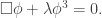
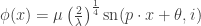
Hera is an integration constant with the dimension of energy, is another integration constant and is the snoidal Jacobi’s elliptic function. Why is this solution so interesting? The reason is that we started with a massless equation and the solution describes a wave with a massive dispersion solution of a free particle! This is the famous mass gap when we translate this result to quantum field theory. I have done this here. So, the classical theory already has the feature of a mass gap. Scalar theory proves to be trivial for the simple reason that we produce, in the low-energy limit, free massive excitations. This is a long awaited result that is going to get increasingly confirmed from other theoretical studies. I will discuss this issue in another post.

What is the relation, if any, between a massless scalar field theory and Yang-Mills theory? Indeed, there exists a deep relation in the low-energy limit, when the coupling becomes increasingly large, as the solutions of the two theories can be mapped. So, for SU(3), mapping theorem shows that

being our solution above provided the substitution . This is a very beautiful result as this gives at once the following conclusions:

• Strong coupling solutions of classical Yang-Mills theory are free massive waves.
• Yang-Mills theory displays massive solutions already at classical level.
• Quantum theory maintains such conclusions as I showed in my papers.

Lattice computations beautifully confirmed this mapping theorem in d=2+1 as showed by Rafael Frigori in a very nice paper (see here). Strong hints are also seen in d=3+1 by other authors and it would be very nice to see an extended computation in this case as the one Frigori did in d=2+1. For yourselves, you can check with Mathematica or Maple the equations given above. You will also see that gauge invariance is not hindered.

Quest for truth



In these days, in Italian theaters and after a two year struggle for distribution, it is possible to see Agora. This is the story of Hypatia,

Hypatia by Raphael

the first female being a scientist and a philosopher. She taught in Alexandria toward the end of the fourth century and the beginning of the fifth. Her struggle against the forces pushing toward Middle Age ended with a failure and she was brutally killed, all her works were burnt and today we know some of her ideas because some of her disciples wrote about that. There is a deep lesson to be learned here. Doing science is a quest for truth but this quest happens inside our world, with forces pushing to avert us from the right track, to stop us again and again or to use us or our ideas for their not so clear aims. So, our community must protect and help gifted people and have their ideas, when we are sure these are correct, spread as soon as possible for the common good and mankind at large. We must avoid to ask ourselves, after sixteen centuries: How many times must Hypatia die again?